GPU computations

In this lesson we will learn how to install ArrayFire and how to use it to perform some computations on GPU.

ArrayFire is a library used to perform array and matrix operations on GPUs. It offers a CUDA, OpenCL and CPU back-end, so you can be sure that your code will be compatible with any machine which can install the ArrayFire binary.

You can find the code for this lesson here.

Installing ArrayFire

In order to use ArrayFire, we need to first install it. You can find the download page here.

Once you have installed the ArrayFire binary, please restart your system. You can now add ArrayFire.jl to your project with the following command:

using Pkg
Pkg.add("ArrayFire")

Using ArrayFire

In order to use ArrayFire, first import the library:

using ArrayFire

You should see a message like this on the REPL:

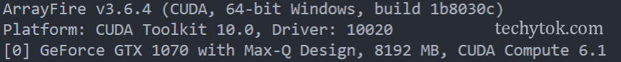
In my case I have an NVidia GPU installed on my PC, thus ArrayFire will use the CUDA back-end.

You can now start using ArrayFire!

When performing computations on GPU we need to take into account that the CPU and GPU don’t have a shared memory, so it is necessary to transfer some data from memory to the GPU and then, after the computation, the results should be sent back to the memory. This operation is usually really slow, so ideally we want to send the starting data to the GPU once and retrieve only the final results.

With ArrayFire it is possible to send some data (usually matrices) to the GPU using the AFArray function. The following code example is taken from the official repository:

# Transfer to device from the CPU
host_to_device = AFArray(rand(100,100))

Some data stored on the GPU can then be transferred back to the memory using the Array function:

# Transfer back to CPU
device_to_host = Array(host_to_device)

Although it is possible to generate a random matrix using the CPU and then you can transfer it to the GPU memory (as seen in the previous example), it is much more convenient and fast to generate the random matrix directly on the GPU:

a = rand(AFArray{Float64}, 100, 100)

Not only we avoid transferring data from memory to the GPU, in this way we will use the rand function provided by ArrayFire, which is highly optimised to work on GPUs.

For further information on the functions available for AFArray, please take a look at the official documentation.

Example: computing π

An example of how it is possible to compute the π is to perform a simple Monte Carlo simulation. In this case we know that the area of a circle is \(A=πr^2\)

If we throw coins at random in a 1x1 square, the probability for a coin to fall inside the inscribed circle is proportional to the area of the circle. Since r=0.5, π is given by:

\[π = 4 \frac{N_{in}}{N_{tot}}\]

On the right side of the equation we have the number of coins that fell inside the circle over the number of total coins thrown.

We can write a simple function to compute π in this way:

using BenchmarkTools

function pi_serial(n)
    inside = 0
    for i in 1:n
        x, y = rand(), rand()
        inside += (x^2 + y^2 <= 1)
    end
    return 4 * inside / n
end

>>>@btime pi_serial(10_000_000)
130.825 ms

It is possible to re-write this function function to work with AFArrays in this way:

using ArrayFire
using BenchmarkTools

function pi_gpu(n)
    return 4 *
           sum(rand(AFArray{Float64}, n)^2 .+ rand(AFArray{Float64}, n)^2 .<= 1) ./
           n
end

Since sum, rand and the matrix operations + and / are able to work on AFArrays, all the computations from line 5 to 7 are performed on the GPU and only the result (a single Float64) is transferred back to the memory. Notice that although we were working with arrays, we didn’t use the broadcasting notation for ^, since ^ for AFArrays is defined to perform the element wise power. If we want to perform the matrix multiplication we need to use *.

Example: Mandelbrot fractal

The Mandelbrot fractal is one of the most famous fractals. For the mathematical definition of the Mandelbrot set, please refer to this Wikipedia article.

In order to numerically compute an image of the Mandelbrot fractal, we take the complex coordinates of each pixels and we compute

\[z_{n+1} = z_{n}^2 + c\] \[z_0 = 0\]

where c is the coordinate of the pixel. We compute z at each iteration and up to the Nth iteration, if at some point \(|(z_n)|>2\) we assign to the pixel the value n, which is the number of iterations required for z to escape. If we then plot the value of each pixel we get the image of the Mandelbrot fractal.

This algorithm can be implemented using ArrayFire in the following way:

using ArrayFire

maxIterations = 500
gridSize = 2048
xlim = [-0.748766713922161, -0.748766707771757]
ylim = [0.123640844894862, 0.123640851045266]

x = range(xlim[1], xlim[2], length = gridSize)
y = range(ylim[1], ylim[2], length = gridSize)

xGrid = [i for i in x, j in y]
yGrid = [j for i in x, j in y]

c = xGrid + im * yGrid

function mandelbrotGPU(c, maxIterations)
    z = c
    count = ones(AFArray{Float32}, size(z))

    for n = 1:maxIterations
        z = z .* z .+ c
        count = count + (abs(z) <= 2)
    end
    return sync(log(count))
end

count = Array(mandelbrotGPU(AFArray(c), maxIterations))

From line 3 to 14 we define the specifications of the fractal: maxIterations is the maximum number of iterations after which we stop the computation of z, gridSize is the size of the image and xlim and ylim define the region of the complex plane where we want to compute the Mandelbrot Set.

From line 16 to 25 we compute the counts for each pixel of the image. At line 17 we assign z = c, since this is the result of the first iteration of the algorithm, at line 18 we initialise the matrix which will contain the counts for each pixel. At line 20 begins the loop to compute z and at line 22 we increment the counter for all the points where abs(z) <= 2.

Usually the computation operations on the GPU are asynchronous and the result is returned only when required, thus before we can return a result we need to call sync to synchronise the computation. At line 24 we require the result of the computation to be synchronised through sync and we return log(count).

At line 27 we call mandelbrotGPUand we move the result of the computation from the GPU to the memory through Array.

We can now plot the result of the computation using Plots and heatmap:

using Plots

heatmap(
    count,
    color = :inferno,
    grid = false,
    colorbar = :none,
    framestyle = :none,
    size = (2048, 2048),
)

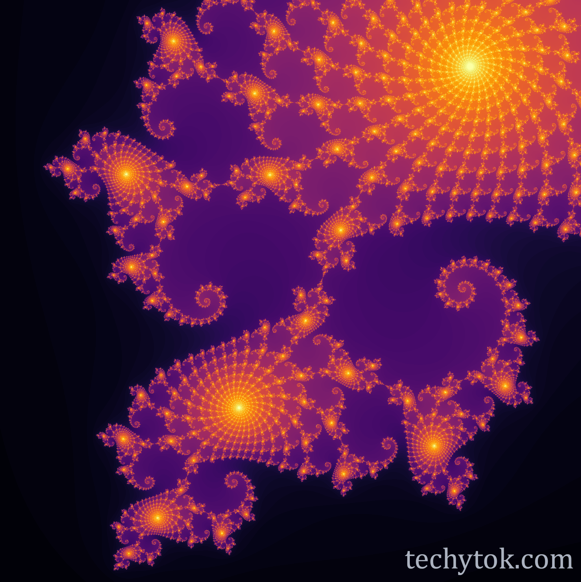
This example was adapted from this code and this package.

CUDA

Although in this guide we have focused on ArrayFire, for compatibility and for its simplicity, it is also possible to write native CUDA kernels using Julia through CuArrays.jl, CUDAnative.jl and CUDAdrv.jl.

We will not deal with the details of how to write CUDA kernels, but libraries like Flux.jl use kernels written in Julia to perform machine learning and achieve high performance in numerical computations.

This is a great example of how Julia can solve the two language problem, since up to a few years ago it was possible to write CUDA kernels only in C++.

The two language problem consists in the need to often write a code first in a language which is easy to write (like Python), in order to get a working prototype, and then rewrite the code in a language which is efficient, like C++. Julia can solve this problem being both easy to write and performant.

Conclusions

In this lesson we have learned how it is possible to use ArrayFire to perform computations on the GPU. Furthermore, we have seen two examples of how to use ArrayFire in concrete applications: computing π and computing the Mandelbrot set. We have then highlighted the possibility to write native CUDA kernels in Julia using a series of packages and how Julia can solve the two language problem in this case.

If you liked this lesson and you would like to receive further updates on what is being published on this website, I encourage you to subscribe to the newsletter! If you have any question or suggestion, please post them in the discussion below!

Thank you for reading this lesson and see you soon on TechyTok!