Code optimisation in Julia

In this guide we will deal with some key points to write efficient Julia code and I will give you some suggestion on how to identify and deal with code bottlenecks.

Although it is not necessary, I suggest you to run this code inside the VSCode IDE with the Julia plugin installed. If you don’t know what VSCode is, I suggest you to take a look at this guide on how to install and use it!

You can find all the code for this guide here.

Julia is fast but it needs your help!

Julia can be extraordinarily fast, but in order to achieve top speed you need to understand what makes Julia fast.

Contrarily to what may seem at first glance, Julia doesn’t draw its speed from type annotations but from type stability. But what are type annotations and what is type stability?

Type annotations

Type annotation are a way to tell Julia the type that a function should expect and they are useful when you plan to write multiple methods (multiple dispatch) for a single function. With type annotations, you can tell a function how to behave according to the type of the arguments that it is given.

For example:

function test1(x::Int)
    println("$x is an Int")
end

function test1(x::Float64)
    println("$x is a Float64")
end

function test1(x)
    println("$x is neither an Int nor a Float64")
end

>>>test1(1)
1 is an Int

>>>test1(1.0)
1.0 is a Float64

>>>test1("techytok")
techytok is neither an Int nor a Float64

But writing a function like:

function test2(x::Int, y::Int)
    return x + y
end

function test2(x::Float64, y::Float64)
    return x + y
end

will not yield a performance gain over simply writing x+y directly and it is not even a good programming practice in Julia, as it would potentially limit the usage of the function with other types which may be supported indirectly.

Julia is pretty good at doing type inference at run-time and will compile the proper code to handle any type of x and y or die trying, in the sense that Julia will tell you that it doesn’t know how to properly handle the type of x and y, so it is better to write code as generic as possible (i.e. without type annotations) and only use them when multiple dispatch is needed or we know that a function can work only with one particular input type.

When you are writing a function which expects a number as an input, it is advisable to use type annotations with Abstract Types, for example using function test(x::Real) instead of writing a method for each concrete type. This way the code will be more readable and more generic, a win-win situation! What’s more, an user who wants to implement a custom number type, if the type is properly defined, will find that your function will work also for their code!

So if it’s not type annotations, which is the first difference which you will spot when comparing for example c++ to python, what makes Julia fast? Roughly said, Julia can compile efficient machine code only if it can infer properly the type of the returned value, which means that your code must be type stable if you want to achieve the maximum possible speed.

Type stability

What does type stability means? It means that the type of the returned value of a function must depend only on the type of the input of the function and not on the particular value it is given.

Take as an example this function:

"""
Returns x if x>0 else returns 0
"""
function test3(x)
    if x>0
        return x
    else
        return 0
    end
end

Let’s type the following code in the REPL:

>>>test3(2)
2

>>>test3(-1)
0

>>>test3(2.0)
2.0

>>>test3(-1.0)
0

Which is a huge problem: as you can see when the input is an Int the return output is always and Int, but when the input is a Float64 (like 2.0 or -1.0), the output may either be a Float64 or an Int. In this case Julia cannot determine beforehand whether the returned value will be a Float64 or an Int, which will ultimately lead to a slower code. In this case the problem may be solved by changing line 6 and writing zero(x) which returns a “zero” of the same type of x.

"""
Returns x if x>0 else returns 0
"""
function test4(x)
    if x>0
        return x
    else
        return zero(x)
    end
end

>>>test4(-1.0)
0.00

In this case it was “easy” to find the bit of code which leads to type instability, but often the code is more complex and so Julia comes in our help with your new best friend, the @code_warntype macro!

What it does is really precious: it tells us if the type of the returned value is unstable and, moreover, it will colour code the result in red if any type instability issue is found. Just call the function with a value which you suspect that may be type unstable and it will do the rest!

>>>@code_warntype test3(1.0)
Body::Union{Float64, Int64} #in red in the REPL
 1 ─ %1 = (x > 0)::Bool
 └──      goto #3 if not %1
 2 ─      return x
 3 ─      return 0

>>>@code_warntype test4(1.0)
Body::Float64 #in blue in the REPL
 1 ─ %1 = (x > 0)::Bool
 └──      goto #3 if not %1
 2 ─      return x
 3 ─ %4 = Main.zero(x)::Core.Compiler.Const(0.0, false)
 └──      return %4

As you can see, in the first case the output is either Float64 or Int, which is not good, and in the second case the output can only be a Float64 (which is good).

In this case Julia may still be able to “recover” from this type instability issue, but if by any chance you see somewhere an ::Any (which will always be marked in red) you will know that there is some serious type instability issue which needs to be fixed. Sometimes fixing type instability is easy, sometimes it is not, you will have to deal with it case by case, but the reward is always great, in my programming experience I have seen a performance gain of a thousand times by fixing type stability issues in my code!

Another common error is changing the type of a variable inside a function:

function test5()
    r=0
    for i in 1:10
        r+=sin(i)
    end
    return r
end

>>>@code_warntype test5()
Variables
 #self#::Core.Compiler.Const(test5, false)
 r::Union{Float64, Int64}
 @_3::Union{Nothing, Tuple{Int64,Int64}}
 i::Int64

 Body::Float64
 1 ─       (r = 0)
 │   %2  = (1:10)::Core.Compiler.Const(1:10, false)
 │         (@_3 = Base.iterate(%2))
 │   %4  = (@_3::Core.Compiler.Const((1, 1), false) === nothing)::Core.Compiler.Const(false, false)
 │   %5  = Base.not_int(%4)::Core.Compiler.Const(true, false)
 └──       goto #4 if not %5
 │         (i = Core.getfield(%7, 1))
 │   %9  = Core.getfield(%7, 2)::Int64
 │   %10 = r::Union{Float64, Int64}
 │   %11 = Main.sin(i)::Float64
 │         (r = %10 + %11)
 │         (@_3 = Base.iterate(%2, %9))
 │   %14 = (@_3 === nothing)::Bool
 │   %15 = Base.not_int(%14)::Bool
 └──       goto #4 if not %15
 3 ─       goto #2
 4 ┄       return r::Float64

As you can see r at the beginning is an Int64 and then is converted into a Float64, which slows down the function. In this case it is enough to declare r=0.00 to solve the problem.

Function profiling

Profiling is the practice of measuing the execution time and memory usage of each part of a piece of code, in order to better understand how to optimise it.

In this section we will learn how to find the bottlenecks in the execution of a function, so that we know which parts of the function should be optimised.

As you probably already know, it is possible to measure the execution time of a function using the @time macro or preferably @btime (which is included in the package BenchmarkTools). They are useful when we want to measure a single function call, but they give no information on what is making a function slow. For this reason we need a tool that enables us to identify which line of code is responsible for the bottleneck.

Luckily there are two exceptional packages which help us in profiling: Profile and the Julia IDE for VSCode. Both of the tools will run the desired function once and will log the execution time of each line of code.

Profile works completely in the REPL and will produce a log file. On the other hand, with the support of VSCode we will be able to display the profiling information in a graph.

Profile

Let’s write two new functions which perform heavy calculations:

function take_a_breath()
    sleep(0.2)
    return
end

function test8()
    r=zeros(100,100)
    take_a_breath()
    for i in 1:100
        A=rand(100,100)
        r+=A
    end
    return r
end

We shall now profile test8:

using Profile
test8()
Profile.clear()
@profile test8()
Profile.print()

If you see a log file extraordinarily long, run line 2 to 4 again as it is possible that you have profiled the compilation of some functions and not test8.

You should see something like:

The number 8 (which may vary) is an indication of how long a function runs. We also have a 1 and a 4, so probably this block is the one responsible for the bottleneck. Profile thus gives you a hint that at line 101 (line 8 of the code snippet) there is a bottleneck: who would have imagined that sleeping for 22ms would have been a slow down?

Unfortunately using Profile.print() is not really user friendly and for this reason VSCode comes in our help!

After having called test8 again, to make sure that the function has been properly compiled, we call the profile viewer macro @profview

test8()
@profview test8()

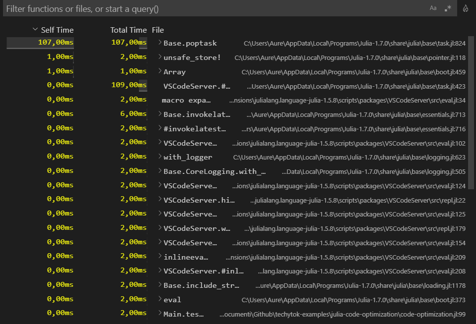
If you have done everything correctly, a new panel should open on the right side of VSCode and you should see something like this:

This list will show you at a glance which are the functions which take more time in your code (in our case, the sleep or wait function) and you can easily evaluate which are the bottlenecks.

It is also possible to display the profiling graphic as a fire graphic. In order to do it, click on the small fire icon on the top right corner of the profiling window (you might have to install an extension). You will see something like this:

In this case, the flame graph is not that informative, since the function is extremely simple, but it is a handy tool when profiling complex functions. The graph should be read from the top to the bottom. The functions on the top usually call the functions under them. If more than one function is involved you will see several branches and the graph will become more complex.

I encourage you to hover your mouse pointer on the functions in the fire graph: you will see the run time of each function involved and you are also able to jump to each function definition. In many cases, the profiler will also add a note on top of the called functions stating how long it took to run them. In order to scroll the flame graph, press ALT and use the scroll wheel, or click and drag the plot. To zoom on a region of the flame graph, point to it and use the scroll wheel.

Tips and Tricks

Now that we have found how to identify type instability issues and how to profile your code, I will give you some tips on how you can make your code faster by changing some little details.

@inbounds

When you are working with for loops and you are sure that the loop condition will not lead to out of bound errors, you can use the @inbounds macro to skip bound checking and gain a speed boost

using BenchmarkTools
arr1=zeros(10000)

function put1!(arr)
    for i in 1:length(arr)
        arr[i]=1.0
    end
end

function put1_inbounds!(arr)
    @inbounds for i in 1:length(arr)
        arr[i]=1.0
    end
end

>>>@btime put1!($arr1)
3.814 μs (0 allocations: 0 bytes)

>>>@btime put1_inbounds!($arr1)
1.210 μs (0 allocations: 0 bytes)

On my PC put1! takes 3.814μs, while put1_inbounds! takes only 1.220μs (which is a noticeable difference).

Static Arrays

When the dimension of an array is known beforehand and it will not change over time, static arrays become incredibly powerful as they enable the compiler to perform advanced optimisations.

They are particularly useful when you need to perform operations (like the sum of the members of an array or matrix operations) on small vectors (<100 elements) or matrices.

If we run the micro benchmark from the official github repository we get something like this:

============================================
    Benchmarks for 3×3 Float64 matrices
============================================
Matrix multiplication               -> 7.4x speedup
Matrix multiplication (mutating)    -> 2.4x speedup
Matrix addition                     -> 31.5x speedup
Matrix addition (mutating)          -> 2.5x speedup
Matrix determinant                  -> 121.2x speedup
Matrix inverse                      -> 70.3x speedup
Matrix symmetric eigendecomposition -> 22.6x speedup
Matrix Cholesky decomposition       -> 7.2x speedup
Matrix LU decomposition             -> 8.4x speedup
Matrix QR decomposition             -> 47.1x speedup
============================================

As you can see the performance gain is enormous!

Matrix indices

When writing performant code, we need to keep in mind how data is stored in the memory. In particular, while in c++ and python matrices are stored in memory in a “row first” manner, in Julia they are stored column first. Which means that when we cycle the indices of a matrix in a nested for loop, if we want to read or write on the matrix, it is better to do so “by column” instead of “by row”.

Here is an example:

arr1 = zeros(100, 200)

@btime for i in 1:100
    for j in 1:200
        arr1[i,j] = 1
    end
end
# 386.600 μs

@btime for j in 1:200
    for i in 1:100
        arr1[i,j] = 1
    end
end
# 380.800 μs

Keyword arguments

When a function is in a critical inner loop, avoid keyword arguments and use only positional arguments, this will lead to better optimisation and faster execution.

function foo1(x,y=2) ... # preferable

function foo2(x; y=2) ... # discouraged inside inner loops

For example, if we define the following functions:

function test_positional(a, b, c)
    return a + b + c
end

function test_keyword(;a, b, c)
    return a + b + c
end

We can see the LLVM code which gets compiled for each one using the @code_llvm macro.

>>>@code_llvm test_positional(1,2,3)

;  @ D:\Users\Aure\Documents\GitHub\techytok-examples\julia-code-optimization\code-optimization.jl:210 within `test_positional'
; Function Attrs: uwtable
define i64 @julia_test_positional_18504(i64, i64, i64) #0 {
top:
; ┌ @ operators.jl:529 within `+' @ int.jl:53
   %3 = add i64 %1, %0
   %4 = add i64 %3, %2
; └
  ret i64 %4
}

@code_llvm test_keyword(a=1,b=2,c=3)

;  @ none within `#test_keyword'
; Function Attrs: uwtable
define i64 @"julia_#test_keyword_18505"({ i64, i64, i64 } addrspace(11)* nocapture nonnull readonly dereferenceable(24)) #0 {
top:
; ┌ @ namedtuple.jl:107 within `getindex'
   %1 = getelementptr inbounds { i64, i64, i64 }, { i64, i64, i64 } addrspace(11)* %0, i64 0, i32 2
   %2 = getelementptr inbounds { i64, i64, i64 }, { i64, i64, i64 } addrspace(11)* %0, i64 0, i32 1
   %3 = getelementptr inbounds { i64, i64, i64 }, { i64, i64, i64 } addrspace(11)* %0, i64 0, i32 0
; └
; ┌ @ D:\Users\Aure\Documents\GitHub\techytok-examples\julia-code-optimization\code-optimization.jl:214 within `#test_keyword#9'
; │┌ @ operators.jl:529 within `+' @ int.jl:53
    %4 = load i64, i64 addrspace(11)* %3, align 8
    %5 = load i64, i64 addrspace(11)* %2, align 8
    %6 = add i64 %5, %4
    %7 = load i64, i64 addrspace(11)* %1, align 8
    %8 = add i64 %6, %7
; └└
  ret i64 %8
}

As you can see, when we call test_keyword there are 9 more lines of code. If test_keyword is a function inside a critical inner loop this will lead to a considerable slowdown.

Avoid global scope variables

As the title says, try to avoid global scope variables as much as you can, as it is more difficult for Julia to optimise them. If possible, try to declare them as const: most of the times a global variable is likely to be a constant, which is a good solution to in part alleviate the problem. When possible, pass all the required data to the function by argument, this way the function will be more flexible and better optimised.

Conclusion

These are some tips and tricks to make your Julia code run faster! The take home message for good performance is keep your code as general as possible and as simple as possible and focus on type stability.

Remember: speed in Julia comes from type stability and not type annotations, which means that you should not use type annotations if not required and that the returned value must depend only on the type of the arguments.

If you liked this lesson and you would like to receive further updates on what is being published on this website, I encourage you to subscribe to the newsletter! If you have any question or suggestion, please post them in the discussion below!

Thank you for reading this lesson and see you soon on TechyTok!