Multiprocessing in Julia: writing a module

In this tutorial I will show you an example of how you can create a module in Julia which implements multiprocessing. We will then see a case example where multiprocessing can be used to speed up physical computations.

Introduction

Multiprocessing is a method of computing in which different parts of a task are distributed between two or more similar central processing units, allowing the computer to complete operations more quickly and to handle larger, more complex procedures.

~merriam-webster.com

This is exactly why we want to implement multiprocessing: let’s suppose we want to compute the value of a function (for example sin(x)) over a series of points (which is an array). In Julia this can be simply done using sin.(x), where x is an array of numbers, but doing so I would only make use of a little part of the computational power which a modern computer have.

In the case where we need to map a function over a series of values (often called an embarrassingly parallel problem) there’s no point in calculating one value at time if we can compute many value in parallel and that’s what we are going to do.

Calculating some values in parallel means that each CPU in our computer gets to compute one value, which means that if we have 4 CPUs we can map our function up to 4 times faster!

I suggest you that you take a look at the official documentation before further delving in this tutorial as I will assume that you have a basic understanding of the available functions. Furthermore I will only deal with distributed for loops, but the techniques described in this simple tutorial can be applied also to more complex modules.

Let’s generate a package

To get started I will show you how you can create a package containing a module.

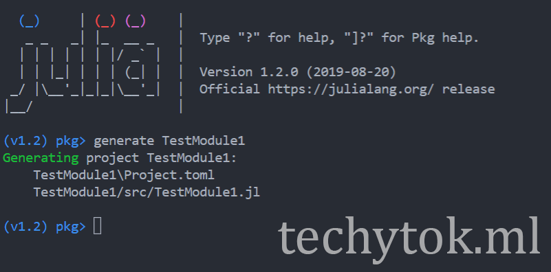
Open the REPL, navigate to the folder of your project and type:

] generate TestModule1

With ] you will open the pkg manager and then you will create a package/project called TestModule1.

Next we need to activate the project typing

activate ./TestModule1

and install the packages needed for this tutorial

add Distributed SharedArrays ProgressMeter Interpolations

Than you can exit the package manager by pressing the backspace.

Create a module

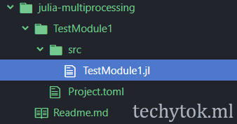
If you take a look at you project structure you will see that a new folder called TestModule1 has been created and that inside the folder src there is a file called TestModule1.jl which is our soon to be Julia module! Open it and modify it as follows:

module TestModule1

export func1, print_nprocs

using Distributed
using SharedArrays
using ProgressMeter
using Interpolations

function func1()
    n = 200000
    arr = SharedArray{Float64}(n)
    @sync @distributed for i = 1:n
        arr[i] = i^2
    end
    res = sum(arr)
    return res
end

function print_nprocs()
    return nworkers()
end

We have defined two functions: func1 and print_nprocs. print_nprocs is pretty straight forward: it prints the number of active workers (i.e. the number of units available for parallel computations). It will be useful in order to check if we have instantiated everything correctly.

func1 creates a SharedArray (i.e. an array which is shared between all the parallel process and which can be modified by each worker) which is filled with n=200000 random values and then it sums the content of the array.

This is not the most efficient way possible to implement the summation, as @distributed can (and should) be used to perform the reduction via @distributed (+) for, but in this way I wouldn’t have the occasion to show you how SharedArrays work.

That’s it, we have implemented a function which uses parallel processing. For such class of problems using distributed computing techniques in Julia is as easy as this! Convenient, don’t you think?

Now that we have created a module which uses parallel processing, we need to call the module from a script and test it!

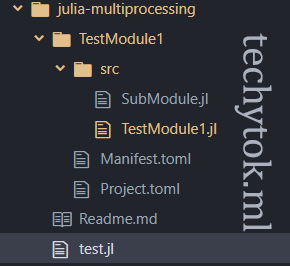
Create a file called test.jl at the root of the project directory. Your project tree should look like this:

In test.jl write the following lines of code:

using Distributed
addprocs(2)

@everywhere using Pkg
@everywhere Pkg.activate("./julia-multiprocessing/TestModule1")

@everywhere using TestModule1

#%%
print_nprocs()

func1()

First we import Distributed, then we add 2 workers (supposing my machine has at least 2 CPU cores).

Now comes the most important part of this guide, which took me a little while to figure out and which is the reason why I decided to write this tutorial.

We need to define the functions/modules which we need to use @everywhere so that they can be used by each worker. We first import Pkg, then we activate the environment @everywhere and import TestModule1 @everywhere (have I already mentioned that you need to define everything @everywhere?)

Aaaand we are ready, let’s call the two functions which we have written and test whether they work as intended!

>>>print_nprocs()
2

>>>func1()
2.6666866667e15

If you follow this work-flow you have to simply write your functions as you would do for “standard” programs and add @distributed where needed to parallelize your loops. You don’t need to focus on which function is defined where, as every function inside the module will be loaded @everywhere.

In the next example let’s create a simple sub module called SubModule.jl and write the following code inside:

module SubMod1
function test_me(x)
    return x^2
end
end

This module can be called inside TestModule1 and we do it by adding the following lines of code:

include("SubModule.jl")
using .SubMod1

function func2()
    n = 100
    arr = SharedArray{Float64}(n)
    @sync @distributed for i = 1:n
        arr[i] = SubMod1.test_me(i)
    end
    res = sum(arr)
    return res
end

This function does nothing in particular (it sums i^2 for i in 1:n), but the point is that it calls an external user defined module, which may be useful when writing your module!

You can call this function by typing TestModule1.func2().

Case study: function interpolation

As I promised in the introduction to this tutorial, we will deal with an example of something that may be useful in physics.

Sometimes you have defined a function which is really expensive to compute and you cannot afford to compute it at each every point or even worse, it is known only in certain points. In this circumstance what you do is create a table of the values of a function and when given an unknown x, interpolate linearly between two subsequent known x.

Let’s consider a highly difficult to compute and exotic function: the sine (I’m joking). Let’s say we can compute it only at certain points. In this example we will use yet another way to map a function over a series of values, which is pmap. pmap is useful when the function to be computed is expensive and will perform load balancing: while @distributedbatches and assign each batch to a worker, pmap will compute each subsequent value on a different worker, which means that if the function execution time may vary considerably from value to value, pmap will require less computation time, even considering the time required to transfer data from the worker back to the main process. If we know that the execution time of each call is pretty much the same for similar x, we can specify the batch_size argument and set it to a greater value, so that each worker will compute more values before the data is moved back to the main process, reducing the data transfer time, at the price of less flexibility on load balancing.

Let’s now create an interpolation table using multiprocessing to speed up the process!

function sine_func(x)
    sleep(22*1e-3)
    return sin(x)
end

function create_interp()
    @info "create_interp"
    x = range(0, stop = 10, length = 1000)

    @info "Computing Interpolation..."
    y = @showprogress pmap(sine_func, x, batch_size=10)


    knots = (x,)
    itp = interpolate(knots, y, Gridded(Linear()))

    return itp
end

This function may look scary at first, but let’s break it down to understand what it does!

sine_func is a wrapper around the sin function which adds a sleep time of 22ms, to simulate an heavy computation.

@info is just a fancy way to say println, but why not?

At line 8 we define the array of points x at which the sine will be computed.

Line 11 is where all the magic happens: first we use the macro @showprogress to create a progress bar which will display the computation status of the parallel map, then we call pmap which will automatically map sine_function over x, taking care of the parallelization, using batch_size=10.

When the parallel computation of the y array is done, we define the knots at line 14 (i.e. the points of the table at which we have computed the function sin(x), and we create the interpolating function (itp) at line 15.

create_interpolation returns a function, which is the interpolating function, so that if we can assign it to a function name and reuse it inside our program. We can do it at compile or evaluation time, it depends on you. I have decided to create the interpolation at compile time, so in my module I add the following lines of code:

const test_interp = create_interp()

and I will be able to call the interpolation from my test.jl script:

test_interp(3.1415)
>>> 9.26375465733916e-5

sin(3.1415)
>>> 9.265358966049026e-5

As you can see the value is not the right one, but it is a good approximation of the true result. The more points you add to the interpolation table, the better accuracy you will achieve.

If you decide to compute the interpolation inside your module, I suggest that you add at the top of the module file __precompile__() (if possible) in order to cache your module and store the interpolation in order to reduce the load time.

You can find the code for this tutorial at https://github.com/aurelio-amerio/techytok-examples/tree/master/julia-multiprocessing

Conclusions

In this tutorial we have learnt how to create a Julia package and how to write a module which uses (simple) parallel computing.

To wrap things up, from this tutorial you have to remember that:

• In this case, you need to call using Distributed and addprocs(n) before calling the module which uses multiprocessing

• You should use n workers, where n is the number of CPU cores you want to use

• You need to activate the environment @everywhere calling:

    @everywhere using Pkg
    @everywhere Pkg.activate(...)
  

  and you need to import the module @everywhere

    @everywhere using TestModule1
  

• When possible, it is better to precompile your module by adding __precompile__() before your module, in order to speed up the loading of your module subsequent times

If you liked this lesson and you would like to receive further updates on what is being published on this website, I encourage you to subscribe to the newsletter! If you have any question or suggestion, please post them in the discussion below!

Thank you for reading this lesson and see you soon on TechyTok!